First, let’s install RelaxiFI (only need to run this once)
Make sure you replace the path (C:/Users/charl/Documents/Python%20dev/RelaxiFI) with the path of the folder where you downloaded RelaxiFI
[2]:
# %pip install RelaxiFI
# %pip install CoolProp
Next import the package
[3]:
import RelaxiFI as relax
import pandas as pd
import numpy as np
import matplotlib.pyplot as plt
[4]:
## Example: find the pressure at 5 km depth

target_depth = 5
crustal_model_config=relax.config_crustalmodel(crust_dens_kgm3=2750)
tolerance = 0.001  # how close you want to be

# run it
pressure = relax.find_P_for_kmdepth(target_depth_km=5, crustal_model_config=crustal_model_config, tolerance=tolerance)
print("Pressure:", pressure)
Pressure: [1.3488749999999998]
[5]:
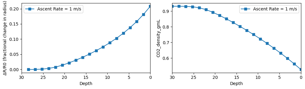
## Let's set the initial conditions
T = 1400 + 273.15  # Temperature in Kelvin

# Radius in m and ascent rate in m/s
R0 = 1 * 10**-6  # Initial value of R (radius of the FI in m)
b=1000*R0 # distance to the crystal edge, Wanamaker uses R0/b=1/1000
ascent_rate_ms=1 #m/s

depth_path_ini_fin_step=[30,0,20] #This defines the starting depth, ending depth and the number of steps in the path. More steps is better, especially for slow ascent rates.

crustal_model_config=relax.config_crustalmodel(crust_dens_kgm3=2750)#the configuration of your crustal model

EOS='SW96' # Equation of state for CO2 (SW96 or SP94)
plotfig=True # Whether to plot the figure or not

resultsSW96 = relax.stretch_in_ascent(R_m=R0, b_m=b,T_K=T,ascent_rate_ms=ascent_rate_ms,crustal_model_config=crustal_model_config,
                                                 depth_path_ini_fin_step=depth_path_ini_fin_step,EOS=EOS,plotfig=plotfig,update_b=False,report_results='fullpath')

resultsSW96
[5]:
| Time(s) | Step | dt(s) | Pexternal(MPa) | Pinternal(MPa) | dR/dt(m/s) | Fi_radius(μm) | b (distance to xtal rim -μm) | ΔR/R0 (fractional change in radius) | CO2_dens_gcm3 | Depth(km) | |
|---|---|---|---|---|---|---|---|---|---|---|---|
| 0 | 0.000000 | 0 | 0.000000 | 809.325000 | 809.325000 | 0.000000e+00 | 1.000000 | 1000.0 | NaN | 0.930837 | 30.000000 |
| 1 | 1578.947368 | 1 | 1578.947368 | 766.728947 | 809.226956 | 1.163351e-14 | 1.000018 | 1000.0 | 0.000018 | 0.930786 | 28.421053 |
| 2 | 3157.894737 | 2 | 1578.947368 | 724.132895 | 808.044271 | 1.404839e-13 | 1.000240 | 1000.0 | 0.000240 | 0.930167 | 26.842105 |
| 3 | 4736.842105 | 3 | 1578.947368 | 681.536842 | 803.138409 | 5.857390e-13 | 1.001165 | 1000.0 | 0.001165 | 0.927591 | 25.263158 |
| 4 | 6315.789474 | 4 | 1578.947368 | 638.940789 | 790.766612 | 1.499037e-12 | 1.003532 | 1000.0 | 0.003532 | 0.921043 | 23.684211 |
| 5 | 7894.736842 | 5 | 1578.947368 | 596.344737 | 768.654713 | 2.760638e-12 | 1.007891 | 1000.0 | 0.007891 | 0.909145 | 22.105263 |
| 6 | 9473.684211 | 6 | 1578.947368 | 553.748684 | 738.266999 | 3.976694e-12 | 1.014170 | 1000.0 | 0.014170 | 0.892363 | 20.526316 |
| 7 | 11052.631579 | 7 | 1578.947368 | 511.152632 | 703.179551 | 4.882372e-12 | 1.021879 | 1000.0 | 0.021879 | 0.872319 | 18.947368 |
| 8 | 12631.578947 | 8 | 1578.947368 | 468.556579 | 666.169342 | 5.531013e-12 | 1.030612 | 1000.0 | 0.030612 | 0.850331 | 17.368421 |
| 9 | 14210.526316 | 9 | 1578.947368 | 425.960526 | 628.609364 | 6.071874e-12 | 1.040199 | 1000.0 | 0.040199 | 0.827035 | 15.789474 |
| 10 | 15789.473684 | 10 | 1578.947368 | 383.364474 | 591.068983 | 6.604244e-12 | 1.050627 | 1000.0 | 0.050627 | 0.802653 | 14.210526 |
| 11 | 17368.421053 | 11 | 1578.947368 | 340.768421 | 553.785570 | 7.179606e-12 | 1.061963 | 1000.0 | 0.061963 | 0.777222 | 12.631579 |
| 12 | 18947.368421 | 12 | 1578.947368 | 298.172368 | 516.874406 | 7.827899e-12 | 1.074323 | 1000.0 | 0.074323 | 0.750704 | 11.052632 |
| 13 | 20526.315789 | 13 | 1578.947368 | 255.576316 | 480.408753 | 8.572585e-12 | 1.087859 | 1000.0 | 0.087859 | 0.723030 | 9.473684 |
| 14 | 22105.263158 | 14 | 1578.947368 | 212.980263 | 444.449960 | 9.437606e-12 | 1.102760 | 1000.0 | 0.102760 | 0.694113 | 7.894737 |
| 15 | 23684.210526 | 15 | 1578.947368 | 170.384211 | 409.059873 | 1.045107e-11 | 1.119262 | 1000.0 | 0.119262 | 0.663863 | 6.315789 |
| 16 | 25263.157895 | 16 | 1578.947368 | 127.788158 | 374.307227 | 1.164810e-11 | 1.137654 | 1000.0 | 0.137654 | 0.632184 | 4.736842 |
| 17 | 26842.105263 | 17 | 1578.947368 | 85.192105 | 340.271870 | 1.307401e-11 | 1.158297 | 1000.0 | 0.158297 | 0.598982 | 3.157895 |
| 18 | 28421.052632 | 18 | 1578.947368 | 42.596053 | 307.047859 | 1.478850e-11 | 1.181647 | 1000.0 | 0.181647 | 0.564170 | 1.578947 |
| 19 | 30000.000000 | 19 | 1578.947368 | 0.000000 | 274.745694 | 1.687140e-11 | 1.208286 | 1000.0 | 0.208286 | 0.527672 | 0.000000 |
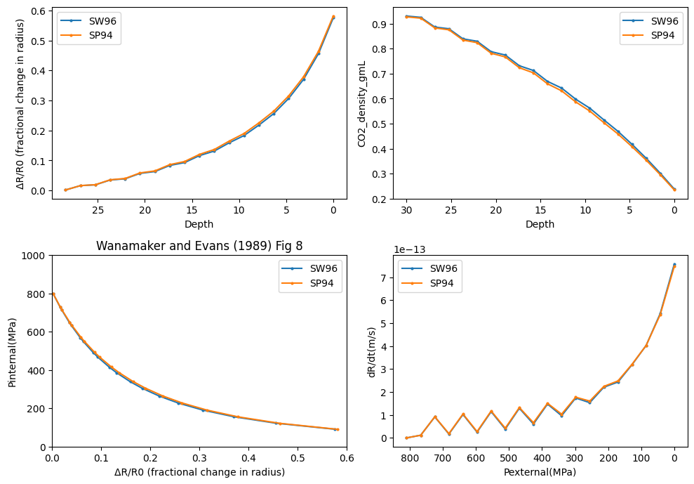
Example, Fig 8 from Wanamaker and Evans 1989
[6]:
## Let's set the initial conditions
T = 1400 + 273.15  # Temperature in Kelvin

# Radius in m and ascent rate in m/s
R0 = 1 * 10**-6  # Initial value of R (radius of the FI in m)
b=1000*R0 # distance to the crystal edge, Wanamaker uses R0/b=1/1000
ascent_rate_ms=0.01 #m/s

depth_path_ini_fin_step=[30,0,20] #This defines the starting depth, ending depth and the number of steps in the path.
crustal_model_config=relax.config_crustalmodel(crust_dens_kgm3=2750)#the configuration of your crustal model

EOS='SW96' # Equation of state for CO2 (SW96 or SP94)
plotfig=False # Whether to plot the figure or not

resultsSW96 = relax.stretch_in_ascent(R_m=R0, b_m=b,T_K=T,ascent_rate_ms=ascent_rate_ms,crustal_model_config=crustal_model_config,
                                                 depth_path_ini_fin_step=depth_path_ini_fin_step,EOS='SW96',plotfig=plotfig)
resultsSP94 = relax.stretch_in_ascent(R_m=R0, b_m=b,T_K=T,ascent_rate_ms=ascent_rate_ms,crustal_model_config=crustal_model_config,
                                                 depth_path_ini_fin_step=depth_path_ini_fin_step,EOS='SP94',plotfig=plotfig)

display(resultsSP94)
display(resultsSW96)
# NOW PLOT - This is the configuration of the plots, can modify x and y vars under 'keys', the first is x the second y

subplot_data = [
    {'data': [resultsSW96, resultsSP94], 'keys': [('Depth(km)', '\u0394R/R0 (fractional change in radius)')], 'xlabel': 'Depth', 'ylabel': '\u0394R/R0 (fractional change in radius)', 'legend': True},
    {'data': [resultsSW96, resultsSP94], 'keys': [('Depth(km)', 'CO2_dens_gcm3')], 'xlabel': 'Depth', 'ylabel': 'CO2_density_gmL', 'legend': True},
    {'data': [resultsSW96, resultsSP94], 'keys': [('\u0394R/R0 (fractional change in radius)', 'Pinternal(MPa)')], 'xlabel': '\u0394R/R0 (fractional change in radius)', 'ylabel': 'Pinternal(MPa)', 'legend': True},
    {'data': [resultsSW96, resultsSP94], 'keys': [('Pexternal(MPa)', 'dR/dt(m/s)')], 'xlabel': 'Pexternal(MPa)', 'ylabel': 'dR/dt(m/s)', 'legend': True}
]

# Make plots
fig, axs = plt.subplots(2, 2, figsize=(10, 7))
axs = axs.flatten()

for ax, subplot in zip(axs, subplot_data):
    for data, label in zip(subplot['data'], ['SW96', 'SP94']):
        for x_key, y_key in subplot['keys']:
            if x_key=='Depth(km)':
                ax.plot(data[x_key], data[y_key], marker='o', markersize=2, label=label)
            else:
                ax.plot(data[x_key], data[y_key], marker='o', markersize=2, label=label)
    ax.set_xlabel(subplot['xlabel'])
    ax.set_ylabel(subplot['ylabel'])
    if subplot.get('legend', False):
        ax.legend()
axs[2].set_title("Wanamaker and Evans (1989) Fig 8")
axs[2].set_xlim(0, 0.6)
axs[2].set_ylim(0, 1000)
axs[0].invert_xaxis()
axs[1].invert_xaxis()
axs[3].invert_xaxis()
plt.tight_layout()
plt.show()
| Time(s) | Step | dt(s) | Pexternal(MPa) | Pinternal(MPa) | dR/dt(m/s) | Fi_radius(μm) | b (distance to xtal rim -μm) | ΔR/R0 (fractional change in radius) | CO2_dens_gcm3 | Depth(km) | |
|---|---|---|---|---|---|---|---|---|---|---|---|
| 0 | 0.000000e+00 | 0 | 0.000000 | 809.325000 | 809.325000 | 0.000000e+00 | 1.000000 | 1000.0 | NaN | 0.927473 | 30.000000 |
| 1 | 1.578947e+05 | 1 | 157894.736842 | 766.728947 | 799.782645 | 1.163351e-14 | 1.001837 | 1000.0 | 0.001837 | 0.922381 | 28.421053 |
| 2 | 3.157895e+05 | 2 | 157894.736842 | 724.132895 | 729.780142 | 9.214945e-14 | 1.016387 | 1000.0 | 0.016387 | 0.883333 | 26.842105 |
| 3 | 4.736842e+05 | 3 | 157894.736842 | 681.536842 | 716.817777 | 1.851318e-14 | 1.019310 | 1000.0 | 0.019310 | 0.875755 | 25.263158 |
| 4 | 6.315789e+05 | 4 | 157894.736842 | 638.940789 | 649.894363 | 1.040974e-13 | 1.035746 | 1000.0 | 0.035746 | 0.834720 | 23.684211 |
| 5 | 7.894737e+05 | 5 | 157894.736842 | 596.344737 | 633.767595 | 2.747294e-14 | 1.040084 | 1000.0 | 0.040084 | 0.824320 | 22.105263 |
| 6 | 9.473684e+05 | 6 | 157894.736842 | 553.748684 | 571.184708 | 1.171408e-13 | 1.058580 | 1000.0 | 0.058580 | 0.781862 | 20.526316 |
| 7 | 1.105263e+06 | 7 | 157894.736842 | 511.152632 | 550.753709 | 4.237659e-14 | 1.065271 | 1000.0 | 0.065271 | 0.767222 | 18.947368 |
| 8 | 1.263158e+06 | 8 | 157894.736842 | 468.556579 | 493.415518 | 1.321885e-13 | 1.086143 | 1000.0 | 0.086143 | 0.723836 | 17.368421 |
| 9 | 1.421053e+06 | 9 | 157894.736842 | 425.960526 | 467.906976 | 6.617173e-14 | 1.096591 | 1000.0 | 0.096591 | 0.703343 | 15.789474 |
| 10 | 1.578947e+06 | 10 | 157894.736842 | 383.364474 | 416.482363 | 1.506234e-13 | 1.120374 | 1000.0 | 0.120374 | 0.659496 | 14.210526 |
| 11 | 1.736842e+06 | 11 | 157894.736842 | 340.768421 | 385.725784 | 1.034832e-13 | 1.136713 | 1000.0 | 0.136713 | 0.631464 | 12.631579 |
| 12 | 1.894737e+06 | 12 | 157894.736842 | 298.172368 | 340.152906 | 1.771635e-13 | 1.164686 | 1000.0 | 0.164686 | 0.587049 | 11.052632 |
| 13 | 2.052632e+06 | 13 | 157894.736842 | 255.576316 | 305.274555 | 1.603108e-13 | 1.189999 | 1000.0 | 0.189999 | 0.550379 | 9.473684 |
| 14 | 2.210526e+06 | 14 | 157894.736842 | 212.980263 | 264.508984 | 2.243525e-13 | 1.225423 | 1000.0 | 0.225423 | 0.504015 | 7.894737 |
| 15 | 2.368421e+06 | 15 | 157894.736842 | 170.384211 | 227.991623 | 2.480374e-13 | 1.264587 | 1000.0 | 0.264587 | 0.458623 | 6.315789 |
| 16 | 2.526316e+06 | 16 | 157894.736842 | 127.788158 | 190.739955 | 3.207595e-13 | 1.315233 | 1000.0 | 0.315233 | 0.407656 | 4.736842 |
| 17 | 2.684211e+06 | 17 | 157894.736842 | 85.192105 | 155.433466 | 4.024152e-13 | 1.378772 | 1000.0 | 0.378772 | 0.353854 | 3.157895 |
| 18 | 2.842105e+06 | 18 | 157894.736842 | 42.596053 | 121.633698 | 5.368188e-13 | 1.463533 | 1000.0 | 0.463533 | 0.295865 | 1.578947 |
| 19 | 3.000000e+06 | 19 | 157894.736842 | 0.000000 | 90.179996 | 7.471906e-13 | 1.581510 | 1000.0 | 0.581510 | 0.234469 | 0.000000 |
| Time(s) | Step | dt(s) | Pexternal(MPa) | Pinternal(MPa) | dR/dt(m/s) | Fi_radius(μm) | b (distance to xtal rim -μm) | ΔR/R0 (fractional change in radius) | CO2_dens_gcm3 | Depth(km) | |
|---|---|---|---|---|---|---|---|---|---|---|---|
| 0 | 0.000000e+00 | 0 | 0.000000 | 809.325000 | 809.325000 | 0.000000e+00 | 1.000000 | 1000.0 | NaN | 0.930837 | 30.000000 |
| 1 | 1.578947e+05 | 1 | 157894.736842 | 766.728947 | 799.600074 | 1.163351e-14 | 1.001837 | 1000.0 | 0.001837 | 0.925726 | 28.421053 |
| 2 | 3.157895e+05 | 2 | 157894.736842 | 724.132895 | 728.515036 | 9.135134e-14 | 1.016261 | 1000.0 | 0.016261 | 0.886866 | 26.842105 |
| 3 | 4.736842e+05 | 3 | 157894.736842 | 681.536842 | 716.381965 | 1.682210e-14 | 1.018917 | 1000.0 | 0.018917 | 0.879949 | 25.263158 |
| 4 | 6.315789e+05 | 4 | 157894.736842 | 638.940789 | 648.525083 | 1.019758e-13 | 1.035018 | 1000.0 | 0.035018 | 0.839517 | 23.684211 |
| 5 | 7.894737e+05 | 5 | 157894.736842 | 596.344737 | 633.266438 | 2.500913e-14 | 1.038967 | 1000.0 | 0.038967 | 0.829981 | 22.105263 |
| 6 | 9.473684e+05 | 6 | 157894.736842 | 553.748684 | 569.584084 | 1.143969e-13 | 1.057030 | 1000.0 | 0.057030 | 0.788156 | 20.526316 |
| 7 | 1.105263e+06 | 7 | 157894.736842 | 511.152632 | 550.260632 | 3.839114e-14 | 1.063092 | 1000.0 | 0.063092 | 0.774750 | 18.947368 |
| 8 | 1.263158e+06 | 8 | 157894.736842 | 468.556579 | 491.799656 | 1.290887e-13 | 1.083474 | 1000.0 | 0.083474 | 0.731843 | 17.368421 |
| 9 | 1.421053e+06 | 9 | 157894.736842 | 425.960526 | 467.474652 | 6.049020e-14 | 1.093025 | 1000.0 | 0.093025 | 0.712826 | 15.789474 |
| 10 | 1.578947e+06 | 10 | 157894.736842 | 383.364474 | 415.107189 | 1.473831e-13 | 1.116296 | 1000.0 | 0.116296 | 0.669168 | 14.210526 |
| 11 | 1.736842e+06 | 11 | 157894.736842 | 340.768421 | 385.365747 | 9.651884e-14 | 1.131536 | 1000.0 | 0.131536 | 0.642493 | 12.631579 |
| 12 | 1.894737e+06 | 12 | 157894.736842 | 298.172368 | 339.239865 | 1.737513e-13 | 1.158970 | 1000.0 | 0.158970 | 0.597939 | 11.052632 |
| 13 | 2.052632e+06 | 13 | 157894.736842 | 255.576316 | 305.022819 | 1.534027e-13 | 1.183192 | 1000.0 | 0.183192 | 0.561964 | 9.473684 |
| 14 | 2.210526e+06 | 14 | 157894.736842 | 212.980263 | 264.156669 | 2.208727e-13 | 1.218066 | 1000.0 | 0.218066 | 0.515063 | 7.894737 |
| 15 | 2.368421e+06 | 15 | 157894.736842 | 170.384211 | 228.010829 | 2.432258e-13 | 1.256471 | 1000.0 | 0.256471 | 0.469263 | 6.315789 |
| 16 | 2.526316e+06 | 16 | 157894.736842 | 127.788158 | 190.945123 | 3.188972e-13 | 1.306823 | 1000.0 | 0.306823 | 0.417084 | 4.736842 |
| 17 | 2.684211e+06 | 17 | 157894.736842 | 85.192105 | 155.897373 | 4.026163e-13 | 1.370394 | 1000.0 | 0.370394 | 0.361691 | 3.157895 |
| 18 | 2.842105e+06 | 18 | 157894.736842 | 42.596053 | 122.277432 | 5.414551e-13 | 1.455887 | 1000.0 | 0.455887 | 0.301641 | 1.578947 |
| 19 | 3.000000e+06 | 19 | 157894.736842 | 0.000000 | 90.863396 | 7.574943e-13 | 1.575491 | 1000.0 | 0.575491 | 0.238027 | 0.000000 |
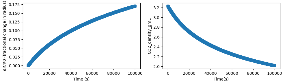
We can also model the stretching of an FI at constant external Pressure (i.e., during storage or quenching)
[7]:
import RelaxiFI as relax
import pandas as pd
import numpy as np
import matplotlib.pyplot as plt

T=1200+273.15
Pinternal=900
Pexternal=0

R0 = 1.0*10**-6  # Initial value of R
b = R0 * 1000  # Value of b
steps = 5000  # Number of steps to iterate
totaltime = 100000

EOS='ideal'
method='Euler'
plotfig=True

solution = relax.stretch_at_constant_Pext(R_m=R0, b_m=b, T_K=T, Pinternal_MPa=Pinternal, Pexternal_MPa=Pexternal,
                                        totaltime_s=totaltime, steps=steps, EOS=EOS,method=method,
                                        plotfig=plotfig)
solution
[7]:
| Time(s) | Step | dt(s) | Pexternal(MPa) | Pinternal(MPa) | dR/dt(m/s) | Fi_radius(μm) | b (distance to xtal rim -μm) | ΔR/R0 (fractional change in radius) | CO2_dens_gcm3 | |
|---|---|---|---|---|---|---|---|---|---|---|
| 0 | 0 | 0 | 0 | 0 | 900.000000 | 4.153999e-12 | 1.000000 | 1000.0 | 0.000000 | 3.233977 |
| 1 | 20 | 1 | 20 | 0 | 899.775721 | 4.153999e-12 | 1.000083 | 1000.0 | 0.000083 | 3.233171 |
| 2 | 40 | 2 | 20 | 0 | 899.551699 | 4.150621e-12 | 1.000166 | 1000.0 | 0.000166 | 3.232366 |
| 3 | 60 | 3 | 20 | 0 | 899.327934 | 4.147250e-12 | 1.000249 | 1000.0 | 0.000249 | 3.231562 |
| 4 | 80 | 4 | 20 | 0 | 899.104424 | 4.143884e-12 | 1.000332 | 1000.0 | 0.000332 | 3.230759 |
| ... | ... | ... | ... | ... | ... | ... | ... | ... | ... | ... |
| 4995 | 99900 | 4995 | 20 | 0 | 560.881724 | 8.878669e-13 | 1.170731 | 1000.0 | 0.170731 | 2.015420 |
| 4996 | 99920 | 4996 | 20 | 0 | 560.856207 | 8.877351e-13 | 1.170749 | 1000.0 | 0.170749 | 2.015329 |
| 4997 | 99940 | 4997 | 20 | 0 | 560.830695 | 8.876033e-13 | 1.170766 | 1000.0 | 0.170766 | 2.015237 |
| 4998 | 99960 | 4998 | 20 | 0 | 560.805188 | 8.874716e-13 | 1.170784 | 1000.0 | 0.170784 | 2.015145 |
| 4999 | 99980 | 4999 | 20 | 0 | 560.779687 | 8.873399e-13 | 1.170802 | 1000.0 | 0.170802 | 2.015054 |
5000 rows × 10 columns
Example, Fig 3 from Wanamaker and Evans 1989
[8]:
T_list = [1300,1350,1400]
temperatures=[t + 273.15 for t in T_list]

Pinternal_values = [900, 200]
Pexternal=0
dataframes = {}

R0 = 1.0e-6  # Initial value of R
b = R0 * 1000  # Value of b
steps = 5000  # Number of steps to iterate
totaltime = 100000

EOS='ideal'
method='Euler'
plotfig=False


for temperature in temperatures:
    for Pinternal in Pinternal_values:
        T = temperature
        solution = relax.stretch_at_constant_Pext(R_m=R0, b_m=b, T_K=T, Pinternal_MPa=Pinternal, Pexternal_MPa=Pexternal,
                                              totaltime_s=totaltime, steps=steps, EOS=EOS,method=method,
                                              plotfig=plotfig)
        key = f"T={temperature-273.15}°C, Pi={Pinternal}"
        dataframes[key] = solution

        if 'T=1300' in key:
            color='yellow'
        if 'T=1350' in key:
            color='orange'
        if 'T=1400' in key:
            color='red'
        if 'Pi=900' in key:
            linestyle='-'
        if 'Pi=200' in key:
            linestyle='--'

        plt.plot(solution['Time(s)'], solution['Fi_radius(μm)'], label=key,color=color,linestyle=linestyle)

plt.xlabel('Time (s)')
plt.ylabel('FI_radius (μm)')
plt.title("Wanamaker and Evans Figure 3")
plt.ylim([1,2.2])
plt.legend()
plt.show()

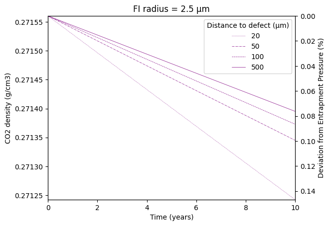
We can then build custom system models as we want
For example here, we model the eruption of an FI of radius 2.5 um trapped at South Caldera Reservoir (Kilaeua) that is stored at Hale’mau’mau reservoir for 10 days
[9]:
####### Establish reservoir PTX conditions
## FI radius
R0 = 2.5 * 10 ** -6 # FI radius in m

## Crustal model crustal_model_configuration
crustal_model_config=relax.config_crustalmodel(crust_dens_kgm3=2750) # You can adjust as you want just call help for details

## Trapping reservoir conditions
Trapping_temp=1300
Trapping_pressure = 1 # in kbar

## surface conditions
Storage_temp=1150  # T in C
Storage_pressure = 0.001 # in kbar

####### Let's start our model

### First let's calculate the CO2 density
fi_rho_initial_gcm3=relax.calculate_rho_for_P_T(EOS='SW96',P_kbar=Trapping_pressure,T_K=Trapping_temp+273.15)[0]

## Now we move the FI to HM reservoir
fi_Pi_storage_initial_MPa=relax.calculate_P_for_rho_T(EOS='SW96',CO2_dens_gcm3=fi_rho_initial_gcm3,T_K=Storage_temp+273.15)['P_MPa'][0]

## Now let's leave it at HM for 10 days
days=10

## Choose equation of state, numerical method and distances to crytal defects

EOS='SW96' # Equation of state for CO2, option SW96, SP94 or ideal

method='RK1' # this is the numerical solver, options are RK1, RK2, RK3 and RK4 (Runge-Kutta)
steps=1000 #number of steps, more is better but slower

dist2defect_list=[20,50,100,500] # Distances to crystal defect structures in microns

T = Storage_temp + 273.15 # T in Kelvin for the model
Pinternal=fi_Pi_storage_initial_MPa
Pexternal=Storage_pressure*100 ##Pressure in MPa for this model

day_in_sec=(24*60*60)
totaltime=days*day_in_sec

## This calculates bvalues for the distances to defect you choose
def calc_multiplier(R0, dist2defect_um):
    multiplier = (dist2defect_um) / (R0 * 10**6)
    return multiplier

R_values = [R0]  # Define R values
b_values= [calc_multiplier(R0, dist)*R0 for dist in dist2defect_list]


# Call the function with appropriate arguments

results_dict_surface = relax.loop_R_b_constant_Pext(R_m_values=R_values, b_m_values=b_values, T_K=T, EOS=EOS, Pinternal_MPa=Pinternal, Pexternal_MPa=Pexternal,
                                                    totaltime_s=totaltime, steps=steps, T4endcalc_PD=Trapping_temp,method=method,
                                              plotfig=False,crustal_model_config=crustal_model_config)


################## Now let's plot our results ######################

# Define some constants and variables
linecolor = 'darkred'
linecolor2 = 'orange'
seconds_in_e_year = 365.25 * 24 * 60 * 60
y_col = 'CO2_dens_gcm3'
x_col = 'Time(s)'
twin_col = 'Calculated depths (km)_TrappingT'
xlabel4plot = 'Time(years)'
ylabel4plot = 'CO2 density (g/cm3)'
twinlabel4plot = 'Calculated depth (km)_TrappingT'
linecolor = 'midnightblue'
linecolor2 = 'purple'
linewidth = 0.5

# Create a figure and axes
fig, ax = plt.subplots()

# Plot the data on the primary y-axis


ax.plot(results_dict_surface['R0']['b0'][x_col] / day_in_sec, results_dict_surface['R0']['b0'][y_col], color=linecolor2, linestyle=':', linewidth=linewidth, label=str(round(b_values[0] * 10 ** 6)))
ax.plot(results_dict_surface['R0']['b1'][x_col] / day_in_sec, results_dict_surface['R0']['b1'][y_col], color=linecolor2, linestyle='-.', linewidth=linewidth, label=str(round(b_values[1] * 10 ** 6)))
ax.plot(results_dict_surface['R0']['b2'][x_col] / day_in_sec, results_dict_surface['R0']['b2'][y_col], color=linecolor2, linestyle='--', linewidth=linewidth, label=str(round(b_values[2] * 10 ** 6)))
ax.plot(results_dict_surface['R0']['b3'][x_col] / day_in_sec, results_dict_surface['R0']['b3'][y_col], color=linecolor2, linestyle='-', linewidth=linewidth, label=str(round(b_values[3] * 10 ** 6)))
ax2 = ax.twinx()

xlim_F=([round(min(results_dict_surface['R0']['b0'][x_col]/day_in_sec)),round(max(results_dict_surface['R0']['b0'][x_col]/day_in_sec))])
ymin_F=np.nanmin([np.nanmin(results_dict_surface['R0']['b0'][y_col])])

ylim_F=[ymin_F,fi_rho_initial_gcm3]

ylim_P_F=relax.calculate_P_for_rho_T(EOS='SW96',CO2_dens_gcm3=pd.Series(ylim_F),T_K=Trapping_temp+273.15)['P_MPa']

ylim_D_F=relax.convert_pressure_to_depth(P_kbar=ylim_P_F/100,
                model='ryan_lerner')


def percent_drop(ylim, original_value):
    return 100-ylim*100/original_value


ax.set_xlim(xlim_F)
ax.set_ylim(ylim_F)
ax2.set_ylim(percent_drop(ylim_P_F,original_value=Trapping_pressure*100))

# Customize axis labels and legends
ax.set_title(f"FI radius = {round(R_values[0]*10**6,1)} μm")
ax.set_xlabel('Time (years)')
ax.set_ylabel(ylabel4plot)
ax2.set_ylabel('Deviation from Entrapment Pressure (%)')

ax.legend(title='Distance to defect (μm)')
[9]:
<matplotlib.legend.Legend at 0x1e52a124210>
[ ]: